Using Excel Filter to Delete or Keep Rows Containing Specific Text or Values

I use Google’s keyword planner all the time but Google will dump everything but the kitchen sink into the relevant key words and I wind up with spreadsheets that are hundreds of rows long. I don’t want to go through each row one by one, though I can tell just by looking at the spreadsheet some types of key words are not what I want.

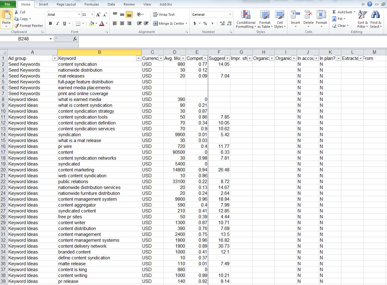
So how do I cut a large spreadsheet down to manageable size, keeping only the rows I want or deleting rows that I definitely don’t want?

The answer is Excel’s Filter tool. (Note: the screenshots and instructions below are for Excel 2010)

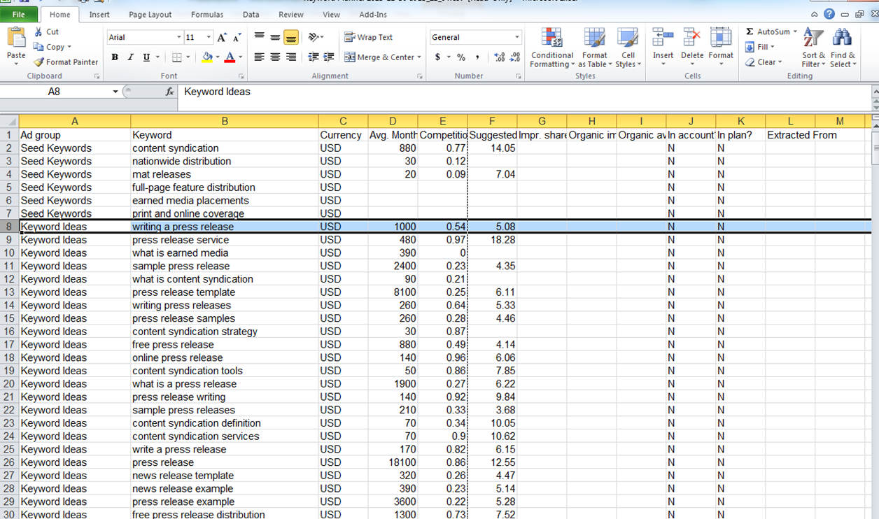
Step 1 – Determine what text or values you want to delete (or keep).

In this case I was looking at keywords related to a specific type of content marketing. However Google delivered up hundreds of keywords related to press releases that I was not interested in.

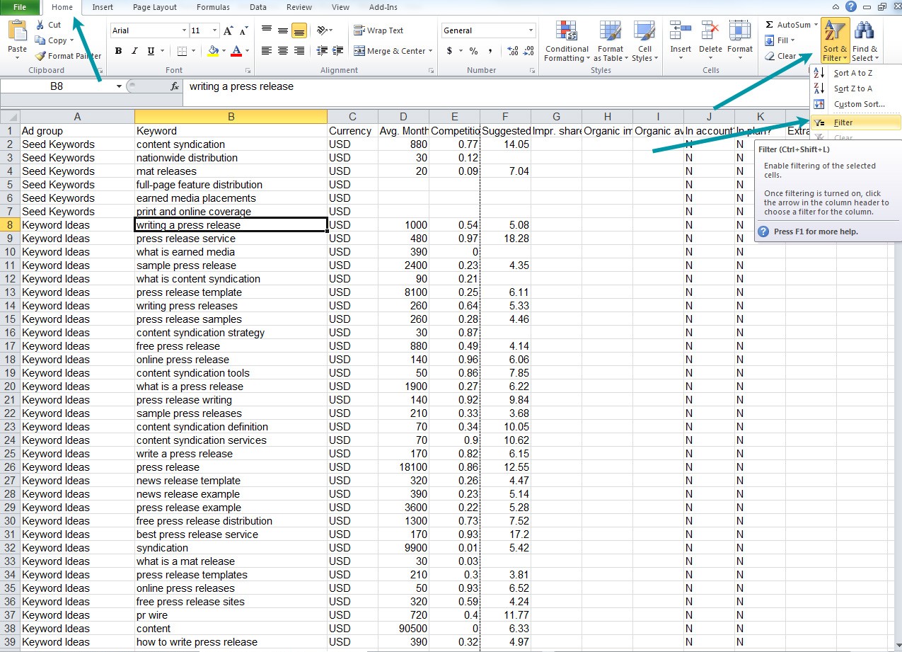
Step 2 – Click on Home tab, select Sort and Filter and then Filter

See the blue arrows below.

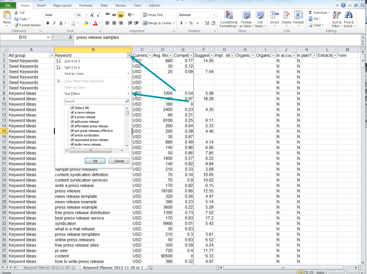
Step 3 – Select the column you want to filter by and then click on Text Filters

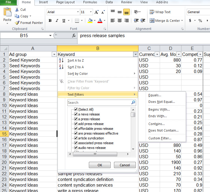
Click on the arrow next to the column that you want to filter. Excel will give you some options including all the values in the in the column you selected.

In my case, I didn’t wanted to filter by a specific value but by all values in the column that are related to the words “press release”. It might be in the beginning, middle or end of the keyword field.

So I clicked on Text Filters.

See the blue arrows below. Before Step 2, you can also start by selecting the column you want to filter by, but that’s not necessary.

Step 4 – Select the type of Text Filter You Want.

When you click on Text Filter, a selection pops up. I know that I want to use “Contains” for my press release filter because it could be anywhere in the field to I click on Contains. But you might want to use Equals especially if you are looking for specific values or other filters.

Step 5 – Add Your Conditions.

You can select up to 2 conditions and you can add wild cards. In this case I could search for “press release” but that would leave out fields with “releases” instead of “release”. So I add the wild card * at the end of press release to search for “press release” and “press releases”. I also know that I don’t want keywords with “news” so I add an “OR” condition for “news”. But you don’t have to add a second condition.

Note that by default the operator for the condition is AND, not OR. So if you make sure to click OR if you want all the rows containing either of your conditions.

Step 6 – Click OK to Filter and Review the Results

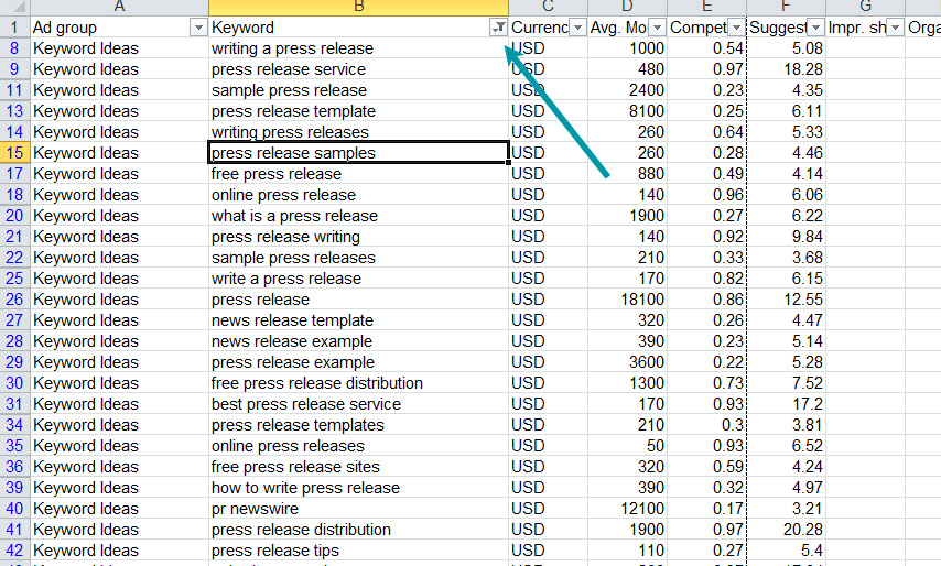
As you can see from some partial results, the filter worked well and captured all the rows with those conditions. Note the little funnel symbol on the column I used to filter to indicate that is filter.

Step 7 – Take Action on Your Filtered Results

You can take whatever actions you want with the results. I wanted to delete them from the spreadsheet. So I selected all of them. You can, of course, leave certain rows out of your selection if you want to keep them.

I selected all the rows I wanted to delete, right clicked, and then selected Delete Row.

Remember to keep the column labels!

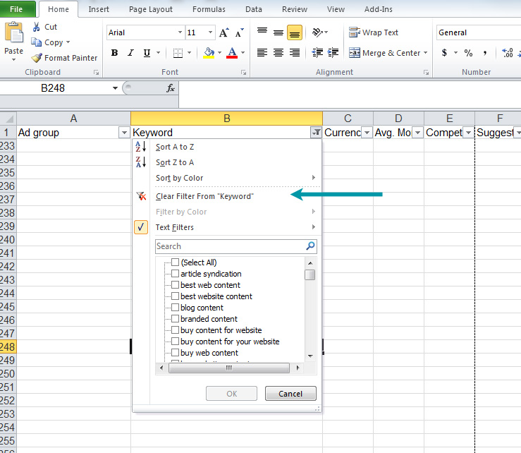
But now I have a blank spreadsheet because my filtered rows are gone.

To view the remaining rows, I need to turn off the filter — or clear the filter.

There are several ways to do this. In the screenshot below I clicked on the funnel icon in the column I filtered by. Then I clicked Clear Filter from Keyword. You can also filter your results further (if you didn’t delete them like I did!)

Results!

I now have a much shorter and cleaner list of keywords to review. However I can already see there are other results that aren’t relevant so it’s back to the filter!